Squad depth is very important in football. It’s why the likes of Manchester City have done so well over the past few years. Erling Haaland has a knock? There’s Julian Alvarez. KDB out? Phil Foden is around. Even in goal: an Ederson absence won’t be felt too much with Stefan Ortega in goal.
The point is, quality on the bench is an integral part of squad building. There are two different kinds of bench player as well: someone that can add something different, and players that can fill in gaps seamlessly. The latter is very important when injuries plague a squad. If your playstyle heavily involves a box poacher and your starting striker gets injured, you don’t want to have to settle for a deep lying forward.
This idea translates to future-proofing your team. A 32-year-old centre back needs an U25 understudy with at least a similar skillset, ready to come in and take the reigns when age inevitably catches up to the veteran.
For a scout or recruitment analyst, this means that being able to find similar players can be an important skill. Principle Component Analysis is one tool that they can use to aid in this process.
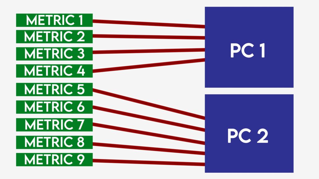
Principal Component Analysis, or PCA, is a mathematical concept that involves dimension reduction. Through linear transformation, a large data set filled with a huge number of variables can be converted into a data set that contains most of the variation within that data into a couple of new variables, called Principal Components (PCs). These PCs are linear combinations of variables in the dataset, accurately weighted to reflect their contribution to variance in the data.
We lose a little bit of precision when doing this, but we are left with a close summary of the data. It’s a bit like taking a book with 100 pages and turning it into a 3-page summary that explains most of the plot. You won’t get all of the side stories and you might lose a small bit of the not-so-important lore behind one or two characters, but you’ll get enough that you could tell the story to someone else.
Let’s use Manchester United as an example of how PCA can be used in football. Casemiro has had a pretty good time at United since joining from Real Madrid last season. However, one key issue has arisen following his first season. When Casemiro isn’t playing, United’s performances drop off. Per 90 minutes, United’s expected goal difference fell by an average of 0.83 when Casemiro wasn’t on the field. Of players that played more than 1,000 minutes for the team last season, only Victor Lindelof and Aaron Wan-Bissaka had a larger impact – and the two often played against weaker opposition as starters were rested.
Casemiro served a few suspensions last season, which meant that United were forced to use Marcel Sabitzer or Scott McTominay in his role. As good as both players are, neither could produce the same amount of quality as the Brazilian, and United suffered for it. On top of that, Casemiro is not young – at 31 years of age, it is more likely that we’ll see a decline in performances from the midfielder as opposed to an improvement. Now is the perfect time for Manchester United to find an understudy for him.
Let’s use PCA to find that understudy.
Firstly, I loaded in data from the 2022-23 season from FBref.com. This included player stats for Europe’s top five leagues. Whilst there may be similar players in lower leagues, it’s also important to take into consideration the level that those players are playing at. After all, there’s no guarantee that a Messi-esque player at Crawley Town would seamlessly fit into a Barcelona side!
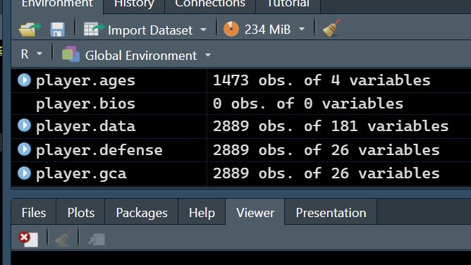
After loading in the data, I was left with a data frame, “player.data”, with 181 variables. Not all these variables were useful. For example, “free kicks taken” wouldn’t be as much of a factor as “passes per 90” when looking at a defensive midfielder’s stylistic output. This is where PCA can help us. I also created a couple of new, style-related variables. Things like possession adjustments and standardisations to 100 touches were made to passes and interceptions amongst other variables, to make sure that the result wasn’t just “players who played for teams that had the same possession as United”.
The next step was conducting the analysis. Doing PCA by hand is a pretty extensive affair. Creating matrices, finding eigenvalues and looking at covariance for a dataset this large would have taken me days. Luckily, in R, all of this can be done in a couple lines of code!

The prcomp() function computes the principal components and returns them. Those principle components have eigenvalues, and based off those values, we can see which of those PCs explain the most variance in the dataset. By scaling the data and putting it into the paran() function, we can use Horn’s method (one of many methods used to evaluate PCs) to see what combination of variables separate the different types of defensive midfielders from each other.
The function suggests that five of the PCs were worth using. Now, we can use those PCs to create similarity scores for all midfielders. Instead of plotting multiple graphs of each PC or writing massive paragraphs explain the details, we can create one number that describes how close a player has played stylistically compared to Casemiro.
To do this, we need to use a measure of distance. For these similarity scores, I used Euclidean distancing. This takes the difference between a player’s and Casemiro’s PCs, squares them and sums them together. I then took the square root of this value and scaled it to a number between 0 and 100 based on that value compared to all the other values.
All I had to do was then sort the dataframe by score, and I was left with this table:
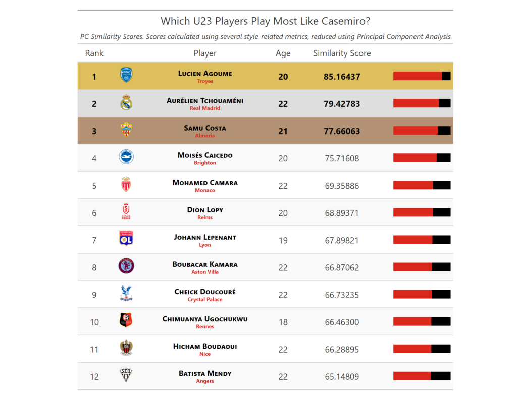
I filtered for players under 23, as this seemed like a good age for development. Looking at the table, some of United’s reported transfer activity makes sense. The past interest in Aurelien Tchouameni, Moises Caicedo and Boubacar Kamara under previous manager Ole Gunnar Solskjaer seems sensible – United could have had a Casemiro-like player years before they did. Perhaps if United did sign one of those two, Ole would still be in a job now…
After constructing a table like this, we can then begin to look at the quality of certain interesting players. Whilst the actual analysis is best left for another article, from this example, I’d flag Lucien Agoume, Johann Lepenant and Cheick Doucoure as players to have a look at.
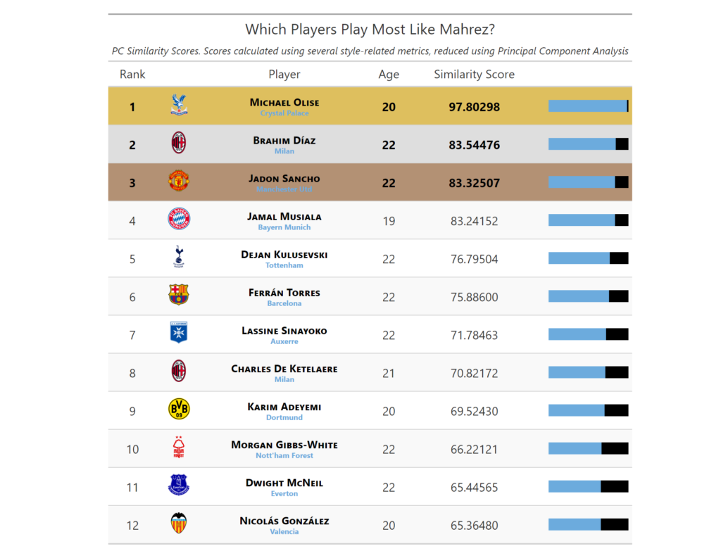
We can use PCA similarity scores to replace players as well. If your star man leaves unexpectedly, you may not have the time to adapt. You need a player who can function the same way as your talisman. For example, Manchester City lost Riyad Mahrez this summer, and were soon linked to Michael Olise. If we look at players who played most like Mahrez last season, those links appear obvious – Olise was far and away the closest winger to the Algerian. When you add other factors like Premier League experience and resale value coming from a young age, the Frenchman was an easy choice for a replacement (City ended up not signing Olise, who signed a new contract with Crystal Palace after a controversial Chelsea approach).
Using these PCA similarity scores is not the only thing a scout should do. As these scores use style-based metrics, we have no idea about the quality of these players. Agoume is the closest to Casemiro in terms of style, but is he, or does he have the potential to be, as good as him? Karim Adeyemi played like Mahrez in the Bundesliga, but Bundesliga matches flow very differently from the Premier League – will his playstyle translate over to England?
As a preliminary step, using Principle Component Analysis can make the shortlisting process more efficient. By only using variables that matter, we can remove the “fluff” in the data and find like-for-like substitutes for other players. It’s a process that I’ve begun to use and hopefully develop over time, but for now, it’s a useful tool that any scout or analyst can add to their arsenal.

